Probability Thoery
There are two kinds of uncertainty, intrinsic uncertainty, aka noise or stochastic uncertainty, & epistemic uncertainty, aka systematic uncertainty. Intrinsic uncertainty, noise, is due to our observations of the world being limited to partial information which can be reduced by gathering different kinds of data. Epistemic uncertainty comes from limitations on the amount of data we have to observe & can be reduced through more data. Even with infinity large data sets to get rid of epistemic uncertainty, we still fail to achieve perfect accuracy due to intrinsic uncertainty.
Probability Theory is a framework that provides tools for consistent quantification & manipulation of uncertainty. Decision Theory allows us to make optimal predictions using this information even in the presence of uncertainty. The frequentist view of statistics defines probability in terms of the frequency of repeatable events. There is another school of thinking about probability that is more general & includes the frequentist perspective as a special case. The use of probability as the quantification of uncertainty is called the Bayesian perspective. It allows us to reason about events that are not repeatable & therefore out of the scope of the frequentist view.
The Rules of Probability
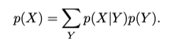
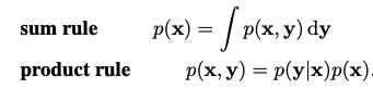
Two simple formulas govern probabilities, the sum rule & the product rule.
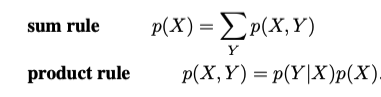
These rules use variables to represent the possibilities of events that are unknown which are therefore called random variables. The following example shows the different kinds of probabilities: joint, conditional, & marginal probabilities.
A Joint probability is the probability of two things happening together, i.e. the probability of x & y which is written like the left hand side of the product rule. A conditional probability is the probability that one event will happen given another event has happened, i.e. the probability of x given y which appears in the product rule & in Bayes' Theorem.
Bayes’ Theorem
By the product rule & symmetry we arrive at Bayes' Theorem which is an important theorem that relates a conditional probability to its reversed conditional probability.
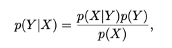
The denominator in Bayes' Theorem can be thought of as a normalization constant there to ensure that the sum over Y will result in a probability of one.
There is an additional interpretation of probabilities from Bayes Theorem as the information before an event occurs & the information after. These are referred to as the prior probability & the posterior probability, i.e. p(X) & p(Y|X).
Independent Variables
If the joint distribution can be factored into the product of marginal probabilities, then the variables in the joint distribution are called independent. The occurrence of one will give us no information about the probability of the other.
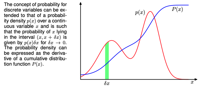
Probability Densities
Probabilities also apply to continuous variables which are known as continuous random variables. We quantify the uncertainty in some prediction by saying, the probability of x falling in to some interval x+dx is equal to the probability density.
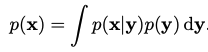
The rules of probability still govern but take on slightly different forms. The second image is the continuous version of Bayes’ Theorem.
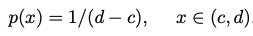
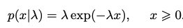
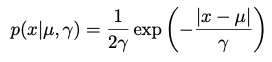
A few examples of probability density distributions are shows below with their corresponding density functions.
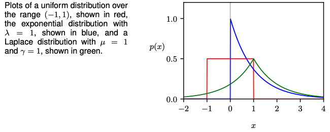
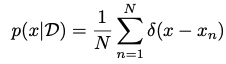
The empirical distribution uses the Dirac delta function to assign all density to a data set, i.e. it integrates to 1. This is accomplished by conditioning many Dirac delta functions on a set of data observations.
Expectation & Covariance
Often, we want to find the weighted average of some function under a probability distribution, i.e. the expectation of a function. The idea applies to discrete & continuous random variables.
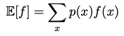
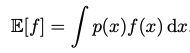
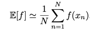
In both cases, given N points from a distribution, we can approximate the expectation by summing over the points & normalizing.
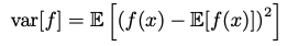
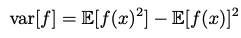
The same idea works with functions of multiple variables & conditional distributions & is denoted by a subscript variable or a conditional bar in the expectation. Variance is a measure of how much a random variable varies around its mean value, i.e. expectation. Variance may also be written in terms of expectations of a function & its square.
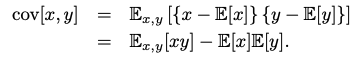
Covariance measures the extent to which two variables move together. A value of zero implies that the variables are independent. In the vector case, covariance is given by a matrix.